Machine Learning Methods
John Hinic 2022-07-21
Machine Learning Methods
Well, we have officially finished learning about several machine learning methods within R. I already knew all of the standard regression techniques, but this was my first time formally learning about the tree-based methods, so that was definitely exciting.
I think the concept of a single regression/classification tree is definitely appealing, but I don’t really see any case that it would be the best method to use - and I have similar thoughts on bagging.
But random forests and boosted trees are both super exciting to me, and they can have really great performance. I think I slightly prefer the random forest method, for a couple main reasons:
- It is a lot easier to understand and explain in my opinion. I think a single tree is relatively intuitive when you show the visual of it to someone, and a random forest model builds off that quite nicely. Single trees can have really high variability, so we can counteract that by fitting lots of trees (i.e., the forest part) that each use a subset of the predictors (i.e., the random part). Then, we simply “average them all together” so to speak.
- The second reason is that it seems slightly easier to tune a random forest model compared to a boosted tree model, although the explainability is definitely a bigger deal to me.
Example
So, we’ll now fit a quick random forest model on the built-in iris
dataset for a demonstration, predicting which species a record belongs
to. We’ll need to load the caret package, and to make the computations
a bit faster we’ll parallelize it using the doParallel package. We’ll
also only use 80% of the data to train the model, then test its
performance on the remaining 20%.
We’ll select the best tuning parameter based on 5-fold, 3-time repeated cross-validation
library(caret)
library(doParallel)
library(tidyverse)

# splitting data
set.seed(9001)
data <- iris %>% mutate(Species = as.factor(Species))
trainIndex <- createDataPartition(data$Species, p = 0.8, list = FALSE)
train <- data[trainIndex, ]
test <- data[-trainIndex, ]

# CV setup
ctrl <- trainControl(method = "repeatedcv", number = 10, repeats = 3)

# parallel setup
cl <- makeCluster(detectCores() - 2)
registerDoParallel(cl)
Now, with the set-up all complete, fitting the model itself is super
simple. We just specify the formula in the train() function as we
normally would, then supply the dataset, model method, relevant tuning
parameters, and any other options we’d like to specify.
rf <- train(
  Species ~ .,
  data = train,
  method = "rf",
  preProcess = c("center", "scale"),
  trControl = ctrl,
  tuneGrid = data.frame(mtry = 1:4)
)
…and that’s it for actually fitting the model.
We can check the accuracy for each of our tuning parameters during the cross-validation, as well as get a plot for the importance of different variables.
rf$results
##   mtry  Accuracy     Kappa AccuracySD   KappaSD
## 1    1 0.9388889 0.9083333 0.07236208 0.1085431
## 2    2 0.9416667 0.9125000 0.07307557 0.1096133
## 3    3 0.9388889 0.9083333 0.07236208 0.1085431
## 4    4 0.9416667 0.9125000 0.07307557 0.1096133
plot(varImp(rf))
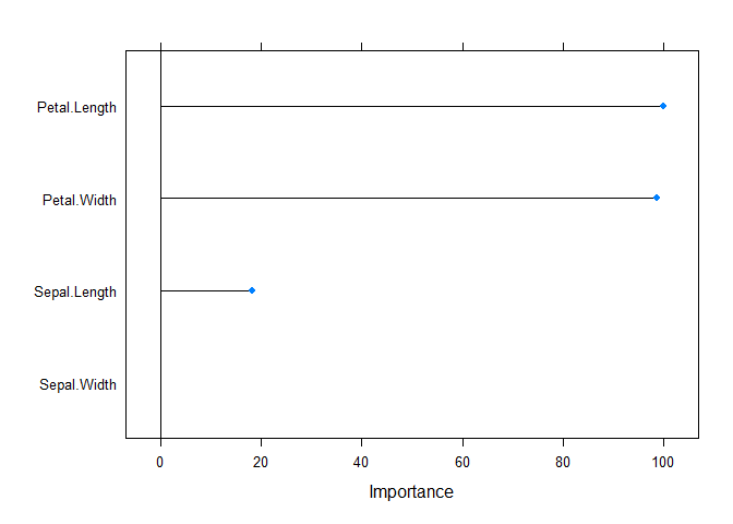
For our tuning parameter, we actually had an exact tie between 2 and 4,
so we will choose 2 just because that is a bit less complex. We can also
see from the variable importance plot, that it seems the petal
width/length are both extremely important, while the sepal measurements
are not nearly so - thus, it makes sense that our mtry value should be
2 instead of 4.
We can also see how our model performs on the test set, as well as create a confusion matrix:
predict(rf, newdata = test) %>%
  confusionMatrix(reference = test$Species)
## Confusion Matrix and Statistics
##
##             Reference
## Prediction   setosa versicolor virginica
##   setosa         10          0         0
##   versicolor      0          9         0
##   virginica       0          1        10
##
## Overall Statistics
##
##                Accuracy : 0.9667
##                  95% CI : (0.8278, 0.9992)
##     No Information Rate : 0.3333
##     P-Value [Acc > NIR] : 2.963e-13
##
##                   Kappa : 0.95
##
##  Mcnemar's Test P-Value : NA
##
## Statistics by Class:
##
##                      Class: setosa Class: versicolor Class: virginica
## Sensitivity                 1.0000            0.9000           1.0000
## Specificity                 1.0000            1.0000           0.9500
## Pos Pred Value              1.0000            1.0000           0.9091
## Neg Pred Value              1.0000            0.9524           1.0000
## Prevalence                  0.3333            0.3333           0.3333
## Detection Rate              0.3333            0.3000           0.3333
## Detection Prevalence        0.3333            0.3000           0.3667
## Balanced Accuracy           1.0000            0.9500           0.9750
stopCluster(cl)
Thus, we can see that the model predicted the correct species for all but 1 record in the test set, which is a pretty solid performance.